The Sound of Climate Change
The audio in this notebook may be loud. Please consider the volume on your machine before playing any audio
Data
In this example, we use the NOAA Global Surface Temperature Dataset (NOAAGlobalTemp), which provides gridded monthly surface temperature anomalies since 1880.
[1]:
import xarray as xr
[2]:
data_path = "data/NOAAGlobalTemp_v5.0.0_gridded_s188001_e202212_c20230108T133308.nc"
ds = xr.open_dataset(data_path)
ds
[2]:
<xarray.Dataset>
Dimensions:  (time: 1716, lat: 36, lon: 72, z: 1)
Coordinates:
  * time     (time) datetime64[ns] 1880-01-01 1880-02-01 ... 2022-12-01
  * lat      (lat) float32 -87.5 -82.5 -77.5 -72.5 -67.5 ... 72.5 77.5 82.5 87.5
  * lon      (lon) float32 2.5 7.5 12.5 17.5 22.5 ... 342.5 347.5 352.5 357.5
  * z        (z) float32 0.0
Data variables:
    anom     (time, z, lat, lon) float32 ...
Attributes: (12/66)
    Conventions:                     CF-1.6, ACDD-1.3
    title:                           NOAA Merged Land Ocean Global Surface Te...
    summary:                         NOAAGlobalTemp is a merged land-ocean su...
    institution:                     DOC/NOAA/NESDIS/National Centers for Env...
    id:                               gov.noaa.ncdc:C00934
    naming_authority:                 gov.noaa.ncei
    ...                              ...
    time_coverage_duration:          P143Y0M
    references:                      Vose, R. S., et al., 2012: NOAAs merged ...
    climatology:                     Climatology is based on 1971-2000 monthl...
    acknowledgment:                  The NOAA Global Surface Temperature Data...
    date_modified:                   2023-01-08T18:33:09Z
date_issued: 2023-01-08T18:33:09ZTo perform our Sonification, we need to first reduce the dimensionality of our data into a one-dimensional time series.
We can achieve this by taking the global average of each grid cell over our desired time dimension (in our case, years)
[3]:
ds_yearly = ds.groupby('time.year').mean()
anom = ds_yearly['anom'].mean(skipna=True, dim=['lat', 'lon', 'z'])
anom
[3]:
<xarray.DataArray 'anom' (year: 143)>
array([-0.3943866 , -0.41972142, -0.4036848 , -0.48530814, -0.57469773,
       -0.5889563 , -0.57268155, -0.5909827 , -0.44562352, -0.38252443,
       -0.63903975, -0.52612305, -0.570924  , -0.59950167, -0.5950165 ,
       -0.5180988 , -0.41718104, -0.44207883, -0.56131285, -0.4545371 ,
       -0.4238661 , -0.46986705, -0.60135543, -0.66082263, -0.72585166,
       -0.5568018 , -0.4936252 , -0.6894805 , -0.72841936, -0.75785506,
       -0.7034879 , -0.75667304, -0.6826453 , -0.65288305, -0.4602562 ,
       -0.43005922, -0.6172296 , -0.71297073, -0.59762526, -0.6004663 ,
       -0.59456426, -0.47546577, -0.5666871 , -0.56307   , -0.5301119 ,
       -0.47914082, -0.38606668, -0.4893744 , -0.4795832 , -0.6426879 ,
       -0.4171341 , -0.38618568, -0.42179072, -0.59395295, -0.39917687,
       -0.45938993, -0.40029082, -0.29080656, -0.2633328 , -0.27344295,
       -0.16464116, -0.11016758, -0.20841345, -0.13299076,  0.01565617,
       -0.13738923, -0.37518796, -0.30405325, -0.35113192, -0.35852575,
       -0.4490882 , -0.32934034, -0.27240175, -0.1811699 , -0.3751917 ,
       -0.43210554, -0.45517403, -0.25939453, -0.23247351, -0.24851352,
       -0.2775711 , -0.22983077, -0.22023346, -0.2538945 , -0.48913643,
       -0.41327626, -0.3905886 , -0.2777611 , -0.34331083, -0.2701262 ,
       -0.2839199 , -0.34365183, -0.3231848 , -0.12641443, -0.37112936,
       -0.2359808 , -0.36379242, -0.06907614, -0.20542464, -0.13779244,
       -0.04034564,  0.06257632, -0.15661713,  0.04536498, -0.12573433,
       -0.14191881, -0.09556889, -0.00960468,  0.07597412, -0.00842201,
        0.1378755 ,  0.09291187, -0.09948993, -0.03128164,  0.00182989,
        0.19177724,  0.01640899,  0.18606322,  0.2912497 ,  0.10348047,
        0.11754002,  0.25927433,  0.31287512,  0.3265392 ,  0.24369767,
        0.38980773,  0.3379023 ,  0.38573822,  0.26357874,  0.31855157,
        0.4427373 ,  0.34472087,  0.38057834,  0.3780964 ,  0.42638323,
        0.5900977 ,  0.727808  ,  0.64048296,  0.5329775 ,  0.67719775,
        0.7383068 ,  0.5341347 ,  0.592656  ], dtype=float32)
Coordinates: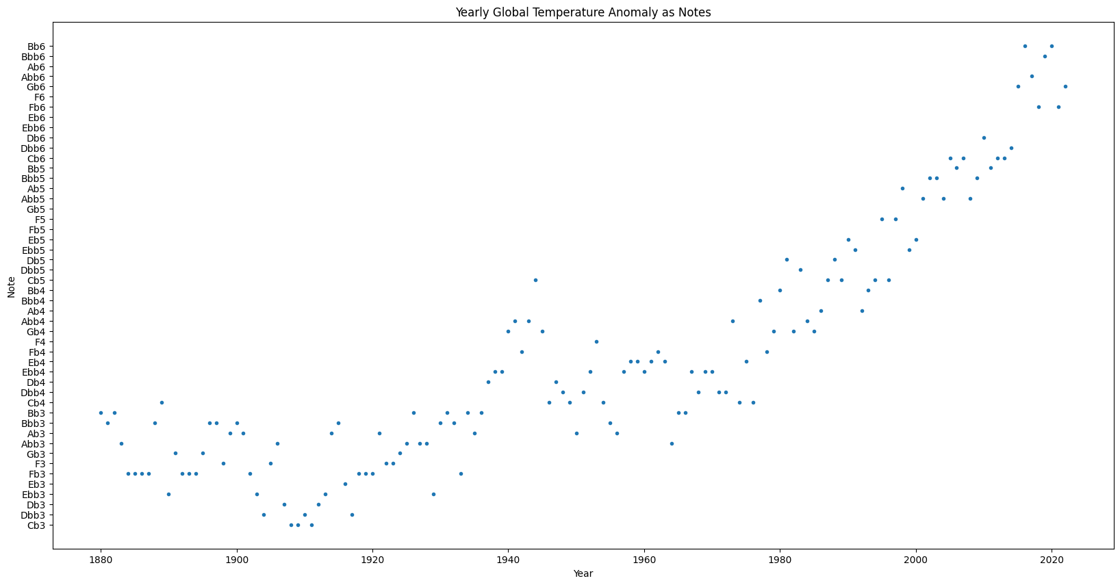
* year (year) int64 1880 1881 1882 1883 1884 ... 2018 2019 2020 2021 2022Sonification
Now that we have a one-dimensional time series, we can perform our sonification.
We first need to specify our SoundMap, which will be used to turn each data point into a musical note.
[4]:
from scisonify.core.soundmaps import DiscreteNoteBins
Here we choose a 3-octave F flat minor scale to be used as our notes
[5]:
smap = DiscreteNoteBins.from_key("Fb:min", octave_range=(3, 6))
Next, we import scisonify.xarray, which will allow us to perform our sonification directly on an Xarray DataArray
[6]:
import scisonify.xarray
[7]:
anom.sonify(note_length=0.1, wave='sine', smap=smap)
[7]:
In addition to listening to our data, we can plot each point as a note to visualize the audio.
[8]:
anom.sonify.plot(x=anom.year,
                 xlabel="Year",
                 marker='o',
                 linewidth=0,
                 ms=3.0,
                 figsize=(20, 10),
                 title="Yearly Global Temperature Anomaly as Notes")
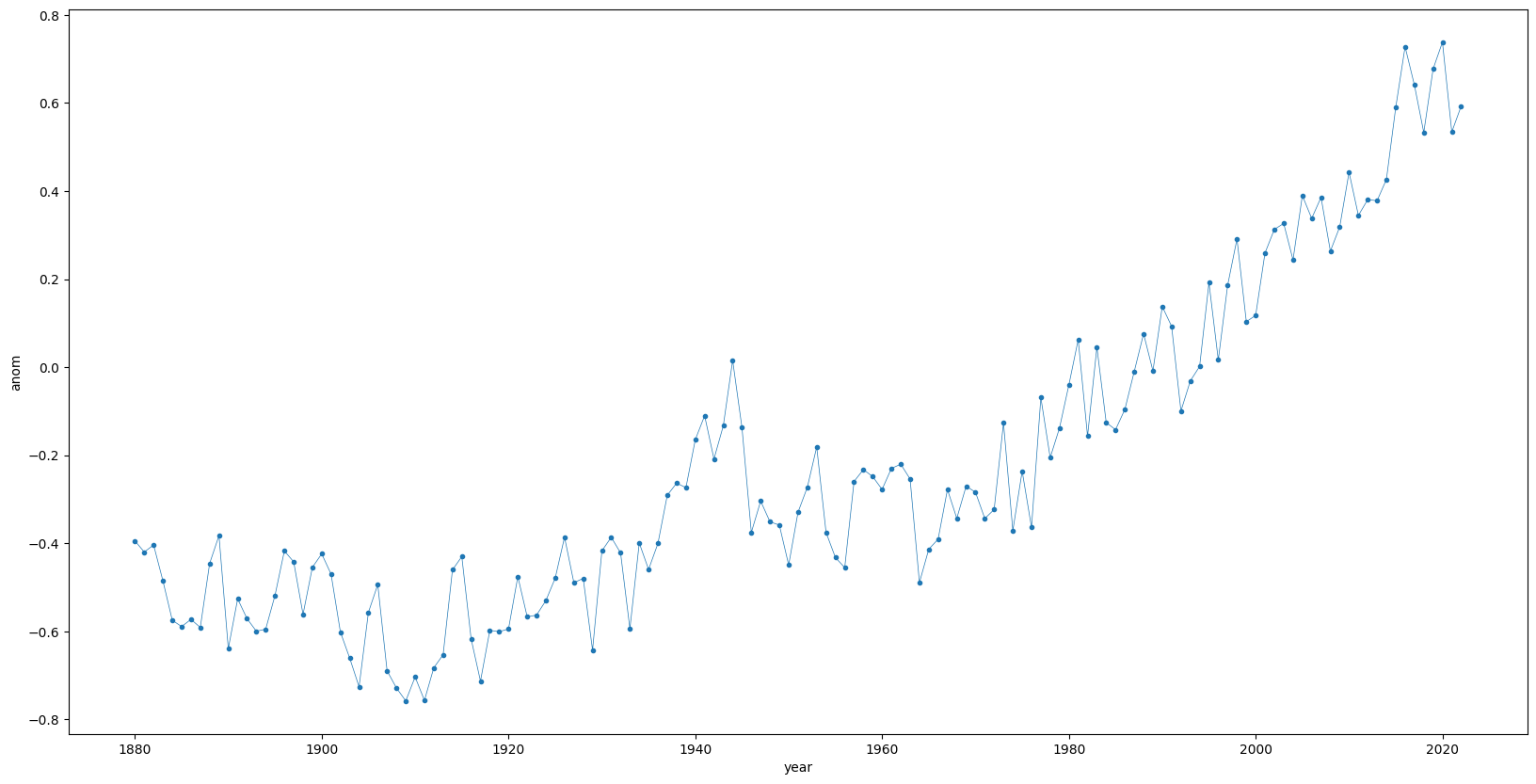
We can compare to this the actual plot of our Temperature anomalies
[9]:
anom.plot(figsize=(20, 10),
          ms=3,
          lw=0.5,
          marker='o')
[9]:
[<matplotlib.lines.Line2D at 0x7ffa0ae86290>]