The Sound of a Transiting Exoplanet

The audio in this notebook may be loud. Please consider the volume on your machine before playing any audio

Data

The data used in this example is taken from the Astropy Time Series Usage Example.

This notebook will not dive into the details about the data, but we will be sonifying the Simple Aperture Photomery Flux (SAP Flux) to listen to the periodic nature of an exoplanet passing in front of its host-star.

The following animation taken from the Planetary Society showcase the dip in brightness that we will be listening for.

from astropy.utils.data import get_pkg_data_filename
from astropy.timeseries import TimeSeries

import numpy as np
from astropy import units as u
from astropy.timeseries import BoxLeastSquares
from astropy.stats import sigma_clipped_stats
from astropy.timeseries import aggregate_downsample
import matplotlib.pyplot as plt
import pandas as pd

filename = get_pkg_data_filename('timeseries/kplr010666592-2009131110544_slc.fits')
ts = TimeSeries.read(filename, format='kepler.fits')

periodogram = BoxLeastSquares.from_timeseries(ts, 'sap_flux')

results = periodogram.autopower(0.2 * u.day)
best = np.argmax(results.power)
period = results.period[best]
transit_time = results.transit_time[best]

mean, median, stddev = sigma_clipped_stats(ts['sap_flux'])
ts['sap_flux_norm'] = ts['sap_flux'] / median
ts_binned = aggregate_downsample(ts, time_bin_size=0.02 * u.day)

WARNING: UnitsWarning: 'BJD - 2454833' did not parse as fits unit: At col 0, Unit 'BJD' not supported by the FITS standard.  If this is meant to be a custom unit, define it with 'u.def_unit'. To have it recognized inside a file reader or other code, enable it with 'u.add_enabled_units'. For details, see https://docs.astropy.org/en/latest/units/combining_and_defining.html [astropy.units.core]
WARNING: UnitsWarning: 'e-/s' did not parse as fits unit: At col 0, Unit 'e' not supported by the FITS standard.  If this is meant to be a custom unit, define it with 'u.def_unit'. To have it recognized inside a file reader or other code, enable it with 'u.add_enabled_units'. For details, see https://docs.astropy.org/en/latest/units/combining_and_defining.html [astropy.units.core]
WARNING: UnitsWarning: 'pixels' did not parse as fits unit: At col 0, Unit 'pixels' not supported by the FITS standard. Did you mean pixel? If this is meant to be a custom unit, define it with 'u.def_unit'. To have it recognized inside a file reader or other code, enable it with 'u.add_enabled_units'. For details, see https://docs.astropy.org/en/latest/units/combining_and_defining.html [astropy.units.core]
WARNING: Input data contains invalid values (NaNs or infs), which were automatically clipped. [astropy.stats.sigma_clipping]
/home/docs/checkouts/readthedocs.org/user_builds/sci-sonify/envs/latest/lib/python3.11/site-packages/astropy/timeseries/downsample.py:31: RuntimeWarning: Mean of empty slice
  result.append(function(array[indices[i] : indices[i + 1]]))
/home/docs/checkouts/readthedocs.org/user_builds/sci-sonify/envs/latest/lib/python3.11/site-packages/astropy/timeseries/downsample.py:32: RuntimeWarning: Mean of empty slice
  result.append(function(array[indices[-1] :]))

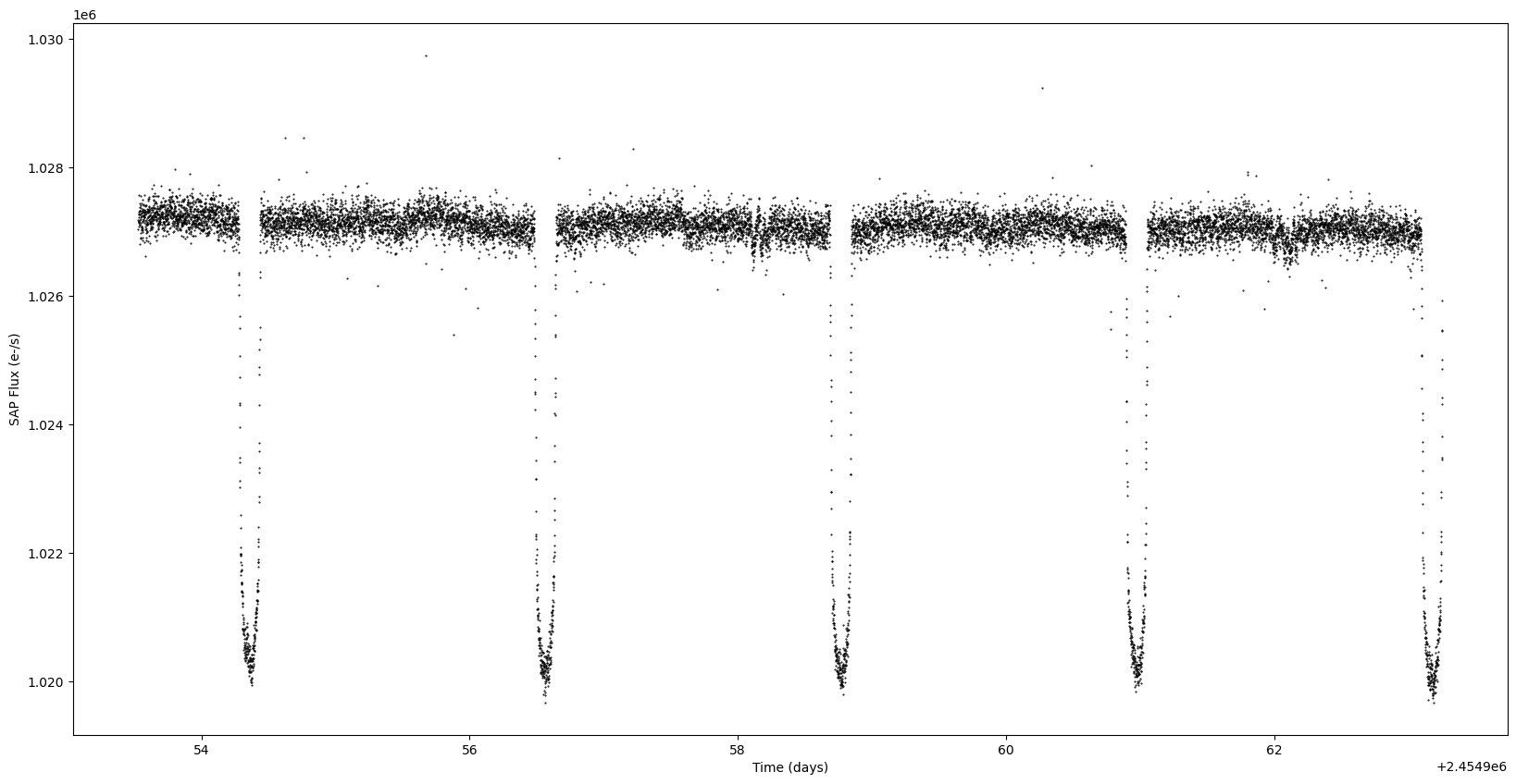
plt.figure(figsize=(20, 10))
plt.plot(ts.time.jd, ts['sap_flux'], 'k.', markersize=1)
plt.xlabel('Time (days)')
plt.ylabel('SAP Flux (e-/s)')

Text(0, 0.5, 'SAP Flux (e-/s)')

plt.figure(figsize=(20, 10))
plt.plot(ts_binned.time_bin_start.jd, ts_binned['sap_flux_norm'], 'k.', markersize=2)
plt.xlabel('Time (days)')
plt.ylabel('SAP Flux (e-/s)')
plt.plot(ts_binned.time_bin_start.jd, ts_binned['sap_flux_norm'], 'r-', drawstyle='steps-post')
plt.xlabel('Time (days)')
plt.ylabel('Normalized flux')

Text(0, 0.5, 'Normalized flux')

Sonification

Since our data is already a one-dimensional time series, there isn’t any further data processing needed.

We will, however, store the values in a Pandas Series to take advantage of the Pandas Sonify Accessor.

import pandas as pd
import scisonify.pandas

sap_flux_norm_binned = pd.Series(ts_binned['sap_flux_norm'].value)
time = ts_binned.time_bin_start.jd

We can now specify our SoundMap, which will be used to turn each data point into a musical note.

from scisonify.core.soundmaps import DiscreteNoteBins

For this example, we will use 2-octave C major scale.

smap = DiscreteNoteBins.from_key("C:maj", octave_range=(3, 4))

Now let’s turn our data in music!

We will be listening for dips in frequencies, which signify the exoplanet passing in front of it’s source star.

Listening to the whole waveform, we can hear the periodic nature of the brightness dips as the planet revolves around it’s star.

sap_flux_norm_binned.sonify(smap=smap, note_length = 0.10)

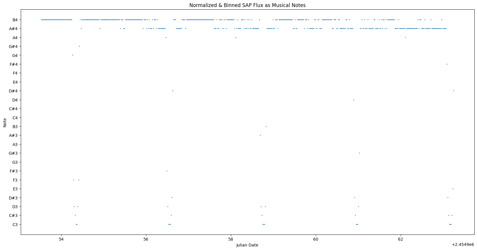
We can plot the data points as musical notes to visually see the musical relationship.

sap_flux_norm_binned.sonify.plot(x=time, ms=1, figsize=(20, 10), title="Normalized & Binned SAP Flux as Musical Notes", xlabel="Julian Date")